
Low-end embedded processors generally lack hardware support for floating-point arithmetic. Although software floating-point implementations are sometimes available in library form, the execution time of the routines tends to be prohibitive. Floating-point representations also consume substantially more data memory than the common integer data types.
Because of these drawbacks, developers tend to avoid floating-point arithmetic in low-end embedded applications and instead implement mathematical operations using integer arithmetic. While the speed and memory advantages of integer arithmetic over floating-point are substantial, it is important to exercise the utmost care in designing integer algorithms. For those coming from the PC development environment (where the use of floating-point is ubiquitous), significant conceptual adjustment may be necessary. This article highlights some integer arithmetic rules of thumb and demonstrates integer algorithm implementation in the context of an example PID cruise control application.
The example code is in C, though many of the concepts discussed here are applicable to other programming languages including assembly.
Signed and Unsigned Integer Types
C offers a variety of signed and unsigned integer data types of various widths. In implementing integer algorithms, the developer must select a specific width for each variable and whether to use a signed or unsigned type.
In situations where it is guaranteed the algorithm input, output and intermediate values are nonnegative under all possible operating conditions, it is appropriate to use unsigned data types throughout. In most designs, however, at least some variables can take on negative values. In the cruise control example we will soon discuss, the speed error (computed as the cruise control speed setting minus the measured vehicle speed) can be positive or negative.
This can cause some difficulty when implementing an algorithm that includes a mix of signed and unsigned variables. An idiosyncrasy of the C language is relevant here: Adding an unsigned int to a signed int produces a result that is an unsigned int. This “usual arithmetic conversion” applies to all the binary operators such as +, – and * as well as to the second and third expressions of the ?: conditional operator. This result is undesirable, to say the least, when implementing an algorithm that operates on negative values. Things happen to work out correctly when the result of the conversion is cast to a signed int in two’s-complement arithmetic, though this is not guaranteed by Standard C and is not portable to non-two’s-complement architectures.
Disaster can occur if the result of a binary operation on mixed-sign integers is assigned to a signed type wider than int. Listing 1 shows an example of this phenomenon on the 16-bit Freescale S12XD processor using the CodeWarrior compiler. The computation assigns 65535 to m instead of -1 as one might naively expect.
    long mixed_add(void)
    {
        int      i = -2;
        unsigned u =  1;
        long     m =  i + u;
        return m; // m = 65535 after the above operations
    }
Listing 1 – Result of adding signed and unsigned integers
Casting the unsigned int to int in each binary operation against an int would produce a signed result, but this defeats the purpose of declaring the variable unsigned in the first place. Instead, I propose a rule of thumb:
Use signed integer types exclusively in arithmetic expressions whenever
any portion of the expression could conceivably be negative.
Under this rule, operations involving positive and negative values of integer types of mixed widths will produce correct results as long as there is no overflow.
Overflow
Overflow occurs when the result of a mathematical operation exceeds the range of the data type receiving the result. For example, adding two N-bit integers can produce a result up to N+1 bits wide. The result of multiplying two N-bit integers can be as much as 2N bits wide.
In many cases, however, information is available to the algorithm designer that guarantees the results of operations will be narrower than these theoretical limits. The designer then chooses the widths of algorithm variables to be as small as possible while ensuring overflow cannot occur.
It is important when making determinations of the expected ranges of computation results to take into account worst-case conditions and to allow some buffer range around those limits. At all times, especially when the system under control enters a stressing and possibly dangerous condition, the control algorithm must accommodate unusual input and intermediate variable excursions without failure.
The designer must keep these concerns in mind when selecting the data type of each variable. In cases where it is a close call to select between, say, a 16-bit integer and a 32-bit integer, the enhanced protection against overflow provided by the wider type tends to outweigh the slight increase in memory usage and processing time.
Designing the Algorithm
Assume a mathematical representation of the algorithm is available. The first step in integer implementation is to identify the algorithm inputs, outputs and intermediate variables. Embedded system inputs often come from an I/O device such as an ADC (analog to digital converter) or pulse counter. Outputs might go to a DAC (digital to analog converter) or PWM (pulse width modulation) device. In each of these cases, the effective width of each algorithm input and output variable is typically defined by the register sizes of the associated I/O devices.
Intermediate processing steps must not result in a loss of precision in the computation from input to output. For instance, if the input signal comes from a 10-bit ADC, all intermediate processing steps must maintain at least 10 bits of precision. More bits of precision in intermediate steps are desirable, as quantization will introduce errors even if 10 bits of precision are maintained throughout. This leads to a second rule of thumb:
The precision of an embedded algorithm implementation should be limited
by the register widths of the I/O devices and not by the software
implementation.
How, in general, does one represent real-world values in units like volts, amps, RPM and the like in integer data types? A popular approach is binary fixed-point, in which a radix point separates the integer part of the number (contained in the higher-order bits) from the fractional part (in the lower-order bits). The LSB (least significant bit) of the integer value in this representation has a value equal to 2n where n is an integer. An example of fixed binary is a signed two’s complement 16-bit integer in which the upper 8 bits contain the sign bit and 7 integer bits while the lower 8 bits contain the fractional part. The maximum value in this representation would be 127.9961 (more precisely, 127 + 255/256) and the minimum would be -128.0000. The LSB in this representation equals 1/256.
While it is conceptually attractive to cleanly separate integer and fractional parts of variables with the binary fixed-point representation, I find this approach to be unnecessarily restrictive. For example, what if my ADC provides voltage readings with a scaling of one LSB = 0.01V? If fixed point binary is in use, it would be necessary to manipulate this value so it has an LSB of 2n. In this case, the nearest value for n would put the LSB at 2-7 = 0.0078125. This scaling can be achieved by multiplying the ADC reading by 32 and then dividing by 25, assuming no overflow. The division results in a slight loss of precision as the 0.01V input LSB does not align with the 0.0078125 fixed-point binary LSB. This has cost us some processing work and has slightly degraded the precision of our input data.
One potential benefit of the binary fixed-point format is that variables with scalings that differ by powers of 2 can be aligned in preparation for addition or subtraction operations by simply performing a shift operation. While this may be a significant benefit if it occurs often enough, in practice there is seldom a need for this. The potential benefits of binary fixed-point scaling are rarely worth the cost of the additional calculations and restrictions on the possible LSB values of integer variables.
Instead, variables that represent input and output values should employ the LSB value that naturally maps to the I/O device. When the LSB is not a power of two, the integer representation will not cleanly separate the integer and fractional parts into separate ranges of bits. This should pose no difficulty. Instead, think of each variable as an integer multiple of its LSB, whatever value that may be.
Intermediate values should have scalings that flow from those of the relevant input and output devices. For example, a voltage reading with an LSB of 0.01V might be multiplied by a current reading with an LSB of 0.05A to yield power. Multiplying the integer values yields power with an LSB of 0.5mW. Unless some consideration such as the possibility of overflow dictates otherwise, it is perfectly appropriate to use this LSB for the intermediate variable. This idea leads to a third rule of thumb:
Intermediate variable scaling should be based on input and output scaling
as much as possible.
This approach maintains the algorithm precision and minimizes the processing required.
It is usually straightforward to select data types for algorithm inputs and outputs based on hardware register sizes. It is less obvious which width is best for intermediate variables of the algorithm. The concerns to be balanced here are the need to maintain the full precision of inputs while guaranteeing overflow cannot occur.
The developer must determine the maximum and minimum possible result of each arithmetic expression. This information should guide the selection of the widths of intermediate variables so memory is not gratuitously wasted and, at the same time, the algorithm operates without overflow or loss of precision under all conceivable conditions.
This leads to the fourth rule of thumb:
Intermediate variable widths must be selected so that overflow cannot occur.
Careful analysis and testing is required to ensure this rule is followed.
PID Cruise Control
We are all familiar with the automotive cruise control. The driver accelerates the vehicle to the desired speed, presses a button to engage the cruise control, releases the accelerator pedal and observes as the control system maintains the speed more or less at the speed at which it was engaged.
Automotive cruise control systems often implement a variation of the PID (proportional, integral, derivative) control algorithm. The input to a PID controller is an error signal, defined in this case as the commanded speed minus the measured speed. The controller’s goal is to drive the error signal to zero. In the case of the cruise control, zero error means the vehicle is traveling at exactly the commanded speed.
The actuator command developed by a PID controller is a weighted sum of the error signal and the integral and derivative of the error signal. Figure 1 shows a PID controller (represented by the Gc block) in a control loop. The Gp block represents the plant to be controlled. In the cruise control application, Gp represents the vehicle drivetrain and motion dynamics with throttle position command (u) as the input and the measured vehicle speed (y) as the output. The commanded speed setting is represented by r and the error signal e = r – y.
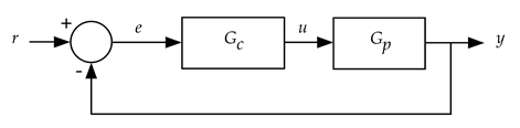
Figure 1 – Block diagram of a system using a PID controller
The Gc block in Figure 1 contains the continuous-time PID control algorithm, which appears in Equation 1. This formula generates an actuator command u given the error signal e. The integral term accumulates the error signal starting from time zero. In the cruise control example, time zero is the moment at which the cruise control is engaged. Kp, Ki and Kd, the PID gains, are constants chosen to optimize controller performance. One or both of the Ki and Kd gains can be set to zero to yield simplified forms of the PID controller. The selection of appropriate values for the Kp, Ki and Kd constants involves an iterative tuning process. See Reference 1 for more information on PID controller tuning.
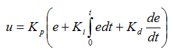
Equation 1 – Continuous-time PID algorithm
To implement the PID algorithm on a digital processor it is necessary to make approximations of the continuous integral and derivative in Equation 1. Equation 2 shows simple approximations that should be adequate as long as the interval between controller updates (h, in units of seconds) is at least ten times shorter than the response time of the system being controlled.

Equation 2 – Discrete approximations of the error integral and derivative
When h is at least ten times shorter than the system’s response time, the system’s response to digital control is similar for most purposes to its response to an analog controller with the same gains. This is an assumption, though, so you must test and verify your implementation to ensure its performance is adequate. One possible problem area is if the input has poor resolution or is noisy, which may result in a derivative estimate from Equation 2 with little relation to the actual derivative. It may be necessary to use more sophisticated estimators than those shown in Equation 2.
In Equation 2, the subscript n indicates the current iteration of the control algorithm. en is the error signal for the current iteration, en-1 is the error signal from the previous iteration, and so on. In the summation approximating the integral, the index i ranges from time zero (when the controller was engaged) to the current iteration.
Using these approximations, equations that generate the next controller output un are shown in Equation 3. The sn term contains the summation of error inputs in Equation 2. To get the algorithm started at n=0, s-1 is initialized to zero and e-1 is set equal to e0. This has the effect of initializing the integral term to zero and setting the initial derivative estimate to zero.
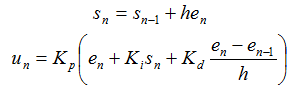
Equation 3 – Discrete-Time PID algorithm
The inputs to Equation 3 consist of the error signal at the current iteration, en, the error signal on the previous iteration, en-1, and the running sum of error measurements computed through the previous iteration, sn-1. The algorithm output is the actuator command un. The en and sn variables must be stored for use on the next iteration.
Implementing the Algorithm
To make things concrete, I’ll provide some numbers to use in this example. I’ll assume the speed error e is derived from a pulse counter vehicle speed input minus the cruise control speed command setting. e has a range of [-1000, 1000] and an LSB of 0.36 km/hr. This range takes into account all conceivable vehicle operating conditions. The output u feeds a PWM device with the input range [0, 255]. Zero represents full-off accelerator and 255 represents full-on accelerator. The algorithm time step h is 0.020 seconds.
Given this information, and assuming the common 8-, 16- and 32-bit signed integer widths are available on the embedded processor, it is clear the input variable e must be at least 16 bits wide while the output u need only be 8 bits wide. Note that u is effectively an unsigned value.
We can now begin implementing Equation 3. The first step is to identify a scaling for h, the algorithm time step in seconds. The most computationally efficient value is to set the LSB of h to 0.020 seconds, which means the equation for sn becomes a simple running sum of the en terms with an LSB equal to 0.36 km/hr * 0.02 sec = 0.36 km/hr * (1000 m/1 km) * (1 hr/3600 sec) * 0.02 sec = 0.002 m.
What might go wrong with the equation for sn? Clearly, if the input en maintains a significant nonzero magnitude for an extended period of time, the sum sn will grow without limit. This condition is unacceptable, and could eventually result in overflow no matter how wide a variable is chosen for sn.
What circumstances might produce such a situation in the cruise control application? Suppose the vehicle is traveling up a long, steep grade and the drivetrain is unable to maintain the commanded speed, even at full throttle. In this situation, the error signal e will maintain a positive value and the sum sn will grow steadily. If sn overflows its integer range, sn will wrap to the largest negative value (assuming two’s-complement arithmetic) and produce a large reduction in the accelerator command signal u. This situation is clearly unacceptable.
In addition, for controller performance reasons, it is undesirable to allow the integral term to grow to large positive or negative magnitudes. If the integral builds to a large magnitude then recovers, the controller output will overshoot the commanded response and slowly converge as the integral diminishes. This undesirable behavior is known as integrator windup.
To prevent excessive overshoot and to avoid the possibility of overflow, it is common to limit the magnitude of the integral term in a PID controller. This limit must be large enough to enable the integral term to do its job of adapting to varying driving conditions. The magnitude limit must also be low enough that intermediate expressions involving the integral (at the positive and negative magnitude limits) cannot overflow. This condition sets an upper bound on the permissible integral magnitude.
Equation 4 shows the steps for computing the limited integrator value. Note that in this equation the time step h is assumed to have an LSB equal to the algorithm time step. It is also required that the integrator limit (MAX_INTEGRATOR) added to the largest possible error signal en cannot cause overflow.
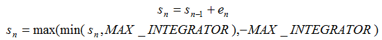
Equation 4 – Limited integral estimate
A similar range analysis applies to the derivative term of the PID algorithm. Cruise control applications seldom use the derivative term (Kd is set to zero and it is unnecessary to estimate the derivative of e) so this analysis is left as an exercise for the reader.
Setting Kd to zero changes the controller to a PI (proportional plus integral) controller with the output equation shown in Equation 5.
![]()
Equation 5 – PI algorithm output equation
The implementation of Equation 5 must guarantee that overflow does not occur in the output. In this example, the right hand side of Equation 5 is a signed result that must be transformed to the unsigned command un. Given the uncertainties in the input to the algorithm, it is difficult to scale the RHS of Equation 5 so it can reach the limits of the range of un and never exceeds those limits.
Instead, it may be preferable to compute a wider signed result for the RHS of Equation 5 that can slightly exceed the limits of un and limit the result to the range of un before writing the output to the PWM register.
Listing 2 shows the full implementation of the PI control algorithm with intermediate variable sizes chosen to meet the design limits given in the code. The TUNED_KP, TUNED_KI and MAX_INTEGRATOR parameter values must be defined during the controller tuning process.
#include <stdint.h>

static const int32_t Kp = TUNED_KP;
static const int32_t Ki = TUNED_KI;
static const int32_t S_lim = MAX_INTEGRATOR;
static int32_t S = 0;

void InitPI(void)
{
	S = 0;
}

uint8_t UpdatePI(int16_t r, int16_t y)
{
	int32_t u;
	int16_t e = r - y;

	S += e;

	if (S > S_lim)
		S = S_lim;
	else if (S < -S_lim)
		S = -S_lim;

	u = Kp * (e + Ki * S);

	if (u > 255)
		u = 255;
	else if (u < 0)
		u = 0;

	return (uint8_t) u;
}
Listing 2 – PI control algorithm using integer math
The example of Listing 2 provides the basic structure for a PI controller implementation. You may find it requires enhancement for a variety of reasons. For example, if you discover your Ki gain needs to have a value of 0.3 then you would need to multiply S by 3 and then divide the result by 10 in line 25. In this example, Ki becomes a ratio of two integers rather than a scalar value.
Conclusion
The use of integer math can provide a vast improvement in execution speed over floating-point in a resource constrained microprocessor. By carefully setting scale factors on each variable you can ensure the range and precision at each processing stage will be adequate
Integer algorithms can provide sufficient precision and margin against overflow if carefully designed. Don’t be afraid to perform math with integers – just do it with care.
References
1. Embedded Control Systems in C/C++, Chapter 2, Jim Ledin, CMP Books, January 2003.